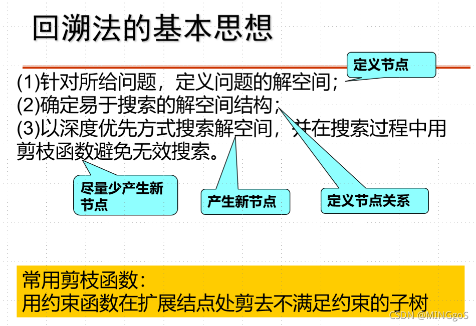
AcWing 842. 排列数字
本题用的算法思想为回溯法
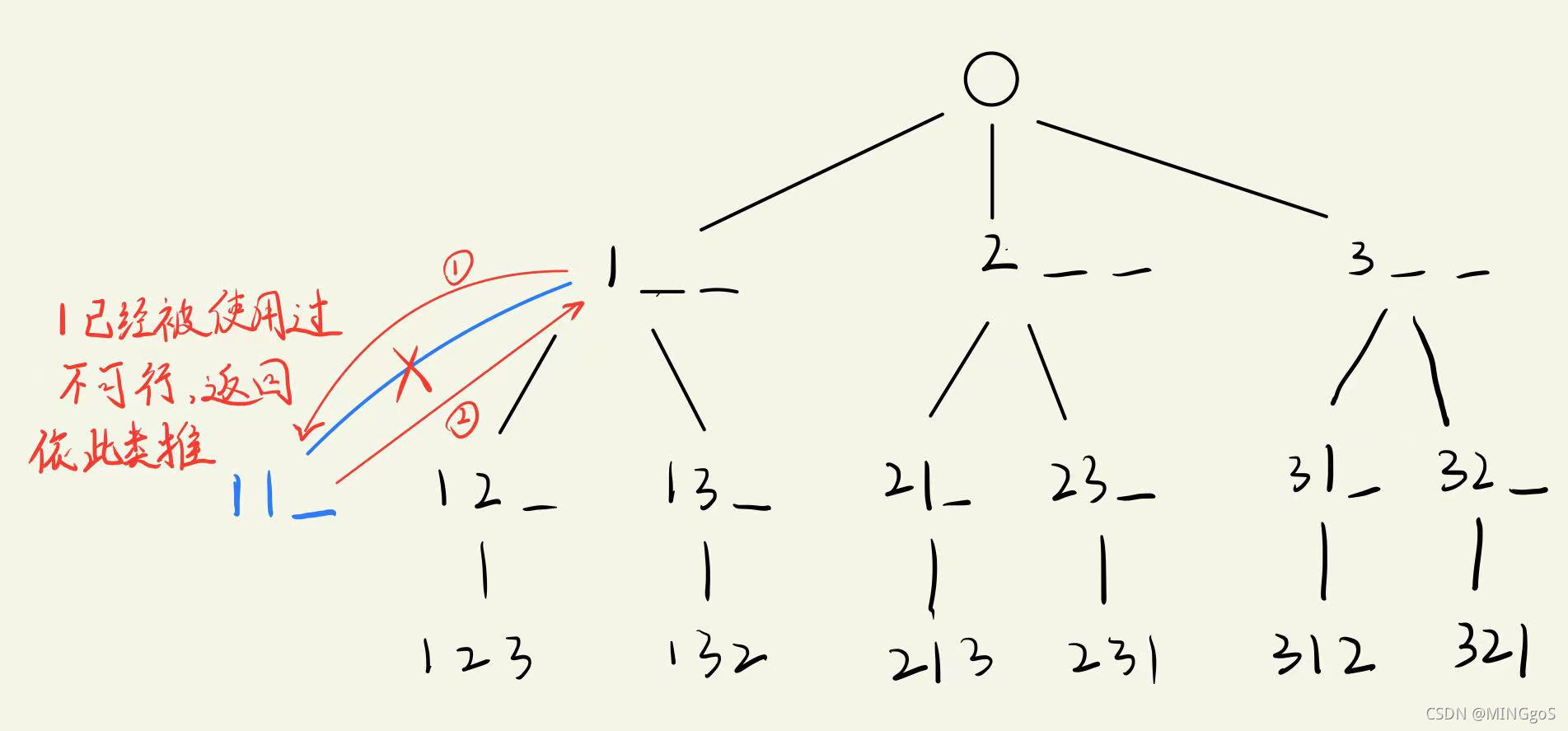
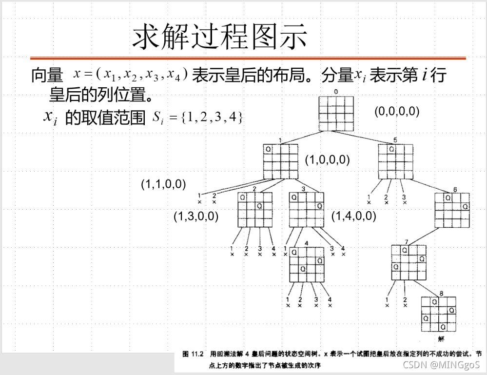
排列数字1,2,3的解空间树:
可行解共有6种
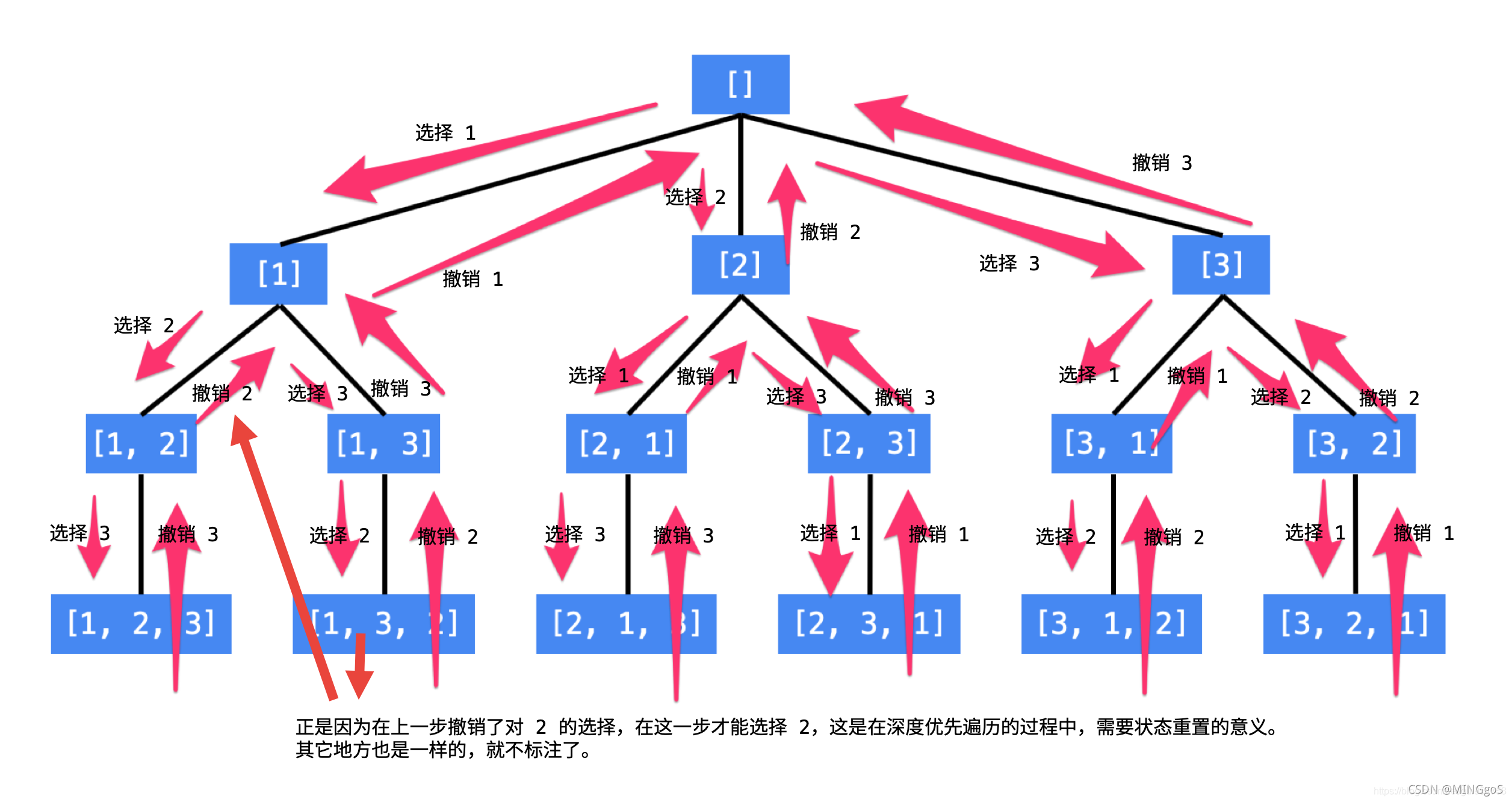
顺序图解:
1
2
3
4
5
6
7
8
9
10
11
12
13
14
15
16
17
18
19
20
21
22
23
24
25
26
27
28
29
30
31
32
33
34
35
| #include<iostream>
using namespace std;
const int N = 10;
int n;
int path[N];
bool st[N];
void dfs(int u)
{
if(u == n)
{
for(int i = 0; i < n; i ++ )
printf("%d ", path[i]);
puts("");
return;
}
for(int i = 1; i <= n; i ++ )
if(!st[i])
{
path[u] = i;
st[i] = true;
dfs(u + 1);
st[i] = false;
}
}
int main()
{
cin >> n;
dfs(0);
return 0;
}
|
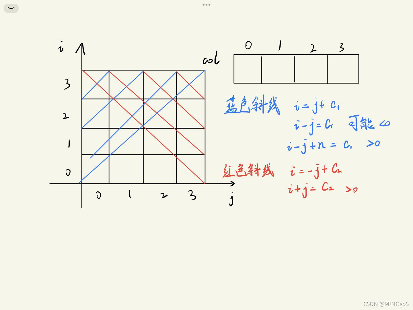
AcWing 843. n-皇后问题
因为每行每列每条对角线都只能有一个皇后,所以可以将各行的皇后映射到同一列上,枚举每列每条对角线是否有皇后。
接着分析,对角线上的皇后。
皇后坐标为(i,j)
- 正对角线映射到一个数组dg中,由于此时
i = j + c1的c1可能为负数,所以需要加上一个偏移量保证c1为正数,用dg[i - j + n] 记录这条正对角线
- 反对角线映射到一个数组udg,此时
i = - j + c2 ,c2必定为正数,用udg[ i + j ]记录这条反对角线
在回溯的过程中只要满足!col[i] && !dg[u - i + n] && !udg[u + i]这个条件就表示当前的坐标能够容纳新的皇后,如此去递归枚举每个位置,找出所有合法的皇后排列即可
1
2
3
4
5
6
7
8
9
10
11
12
13
14
15
16
17
18
19
20
21
22
23
24
25
26
27
28
29
30
31
32
33
34
35
36
37
38
39
| #include<iostream>
using namespace std;
const int N = 20;
int n;
char g[N][N];
bool col[N], dg[N], udg[N];
void dfs(int u)
{
if(u == n)
{
for(int i = 0; i < n; i ++ ) puts(g[i]);
puts("");
return;
}
for(int i = 0; i < n; i ++ )
{
if(!col[i] && !dg[u + i] && !udg[n - u + i])
{
g[u][i] = 'Q';
col[i] = dg[u + i] = udg[n - u + i] = true;
dfs(u + 1);
col[i] = dg[u + i] = udg[n - u + i] = false;
g[u][i] = '.';
}
}
}
int main()
{
cin >> n;
for(int i = 0; i < n; i ++ )
for(int j = 0; j < n; j ++ )
g[i][j] = '.';
dfs(0);
return 0;
}
|
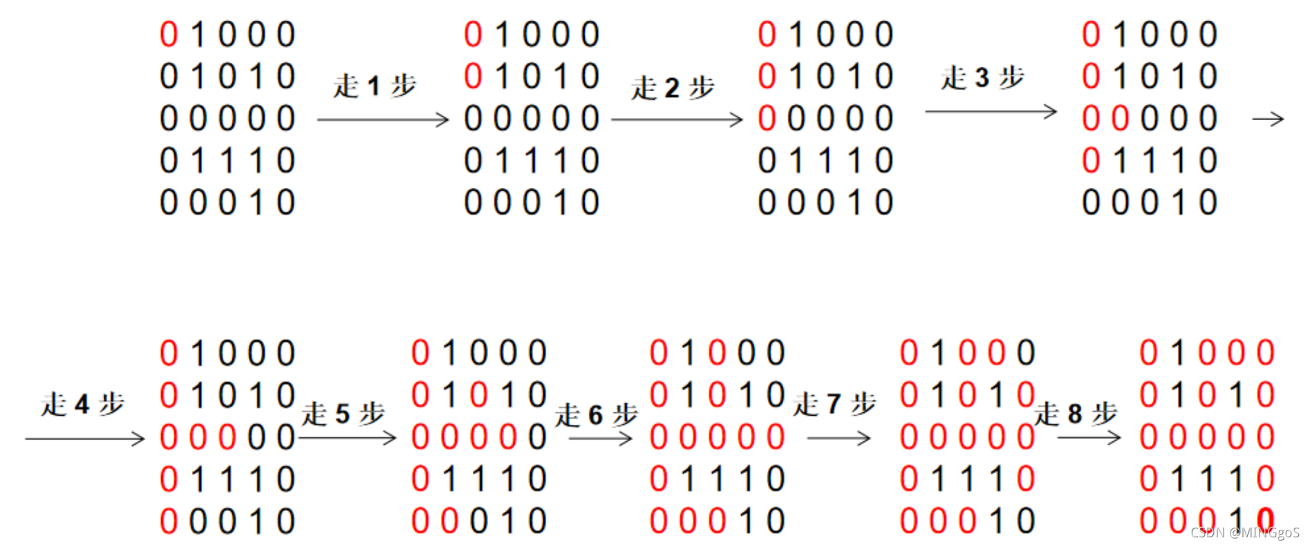
AcWing 844. 走迷宫
引用自深度优先搜索和广度优先搜索的深入讨论
(一)深度优先搜索的特点是:
(1)无论问题的内容和性质以及求解要求如何不同,它们的程序结构都是相同的,即都是深度优先算法(一)和深度优先算法(二)中描述的算法结构,不相同的仅仅是存储结点数据结构和产生规则以及输出要求。
(2)深度优先搜索法有递归以及非递归两种设计方法。一般的,当搜索深度较小、问题递归方式比较明显时,用递归方法设计好,它可以使得程序结构更简捷易懂。当搜索深度较大时,当数据量较大时,由于系统堆栈容量的限制,递归容易产生溢出,用非递归方法设计比较好。
(3)深度优先搜索方法有广义和狭义两种理解。广义的理解是,只要最新产生的结点(即深度最大的结点)先进行扩展的方法,就称为深度优先搜索方法。在这种理解情况下,深度优先搜索算法有全部保留和不全部保留产生的结点的两种情况。而狭义的理解是,仅仅只保留全部产生结点的算法。本书取前一种广义的理解。不保留全部结点的算法属于一般的回溯算法范畴。保留全部结点的算法,实际上是在数据库中产生一个结点之间的搜索树,因此也属于图搜索算法的范畴。
(4)不保留全部结点的深度优先搜索法,由于把扩展望的结点从数据库中弹出删除,这样,一般在数据库中存储的结点数就是深度值,因此它占用的空间较少,所以,当搜索树的结点较多,用其他方法易产生内存溢出时,深度优先搜索不失为一种有效的算法。
(5)从输出结果可看出,深度优先搜索找到的第一个解并不一定是最优解。
二、广度优先搜索法的显著特点是:
(1)在产生新的子结点时,深度越小的结点越先得到扩展,即先产生它的子结点。为使算法便于实现,存放结点的数据库一般用队列的结构。
(2)无论问题性质如何不同,利用广度优先搜索法解题的基本算法是相同的,但数据库中每一结点内容,产生式规则,根据不同的问题,有不同的内容和结构,就是同一问题也可以有不同的表示方法。
(3)当结点到跟结点的费用(有的书称为耗散值)和结点的深度成正比时,特别是当每一结点到根结点的费用等于深度时,用广度优先法得到的解是最优解,但如果不成正比,则得到的解不一定是最优解。这一类问题要求出最优解,一种方法是使用后面要介绍的其他方法求解,另外一种方法是改进前面深度(或广度)优先搜索算法:找到一个目标后,不是立即退出,而是记录下目标结点的路径和费用,如果有多个目标结点,就加以比较,留下较优的结点。把所有可能的路径都搜索完后,才输出记录的最优路径。
(4)广度优先搜索算法,一般需要存储产生的所有结点,占的存储空间要比深度优先大得多,因此程序设计中,必须考虑溢出和节省内存空间得问题。
(5)比较深度优先和广度优先两种搜索法,广度优先搜索法一般无回溯操作,即入栈和出栈的操作,所以运行速度比深度优先搜索算法法要快些。
总之,一般情况下,深度优先搜索法占内存少但速度较慢,广度优先搜索算法占内存多但速度较快,在距离和深度成正比的情况下能较快地求出最优解。因此在选择用哪种算法时,要综合考虑。决定取舍。
走迷宫过程图解:
1
2
3
4
5
6
7
8
9
10
11
12
13
14
15
16
17
18
19
20
21
22
23
24
25
26
27
28
29
30
31
32
33
34
35
36
37
38
39
40
41
42
43
44
45
46
47
48
49
50
51
52
53
54
55
56
57
58
59
60
| #include<iostream>
#include<algorithm>
#include<string.h>
#define x first
#define y second
using namespace std;
const int N = 110;
typedef pair<int, int> PII;
int n, m;
int g[N][N];
int d[N][N];
PII q[N * N];
int bfs()
{
int hh = 0, tt = 0;
q[0] = {0, 0};
memset(d, -1, sizeof d);
d[0][0] = 0;
int dx[4] = {-1, 0, 1, 0};
int dy[4] = {0, 1, 0, -1};
while(hh <= tt)
{
auto t = q[hh ++ ];
for(int i = 0; i < 4; i ++ )
{
int a = t.x + dx[i], b = t.y + dy[i];
if(a < 0 || a >= n || b < 0 || b >= m)
continue;
if(g[a][b] == 0 && d[a][b] == -1)
{
d[a][b] = d[t.x][t.y] + 1;
q[ ++ tt] = {a, b};
}
}
}
return d[n - 1][m - 1];
}
int main()
{
cin >> n >> m;
for(int i = 0; i < n; i ++ )
for(int j = 0; j < m; j ++ )
cin >> g[i][j];
cout << bfs() << endl;
return 0;
}
|
STL版本
1
2
3
4
5
6
7
8
9
10
11
12
13
14
15
16
17
18
19
20
21
22
23
24
25
26
27
28
29
30
31
32
33
34
35
36
37
38
39
40
41
42
43
44
45
46
47
48
49
| #include<iostream>
#include<algorithm>
#include<queue>
#include<string.h>
using namespace std;
const int N = 110, M = 110;
typedef pair<int, int> PII;
queue<PII> que;
int n, m;
int g[N][N];
int d[N][N];
int bfs()
{
que.push({0, 0});
memset(d, -1, sizeof d);
d[0][0] = 0;
int dx[4] = {-1, 0, 1, 0}, dy[4] = {0, 1, 0, -1};
while(!que.empty())
{
auto t = que.front();
que.pop();
for(int i=0; i<4; i++)
{
int x = t.first + dx[i], y = t.second + dy[i];
if(x >= 0 && x < n && y >= 0 && y < m && g[x][y] == 0 && d[x][y] == -1)
{
d[x][y] = d[t.first][t.second] + 1;
que.push({x, y});
}
}
}
return d[n-1][m-1];
}
int main()
{
cin >> n >> m;
for(int i=0; i<n; i++)
for(int j=0; j<m; j++)
cin >> g[i][j];
cout << bfs() << endl;
return 0;
}
|
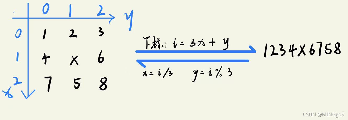
AcWing 845. 八数码
求最少操作步数,若无法变换则返回-1
可以利用BFS求出最小交换步数
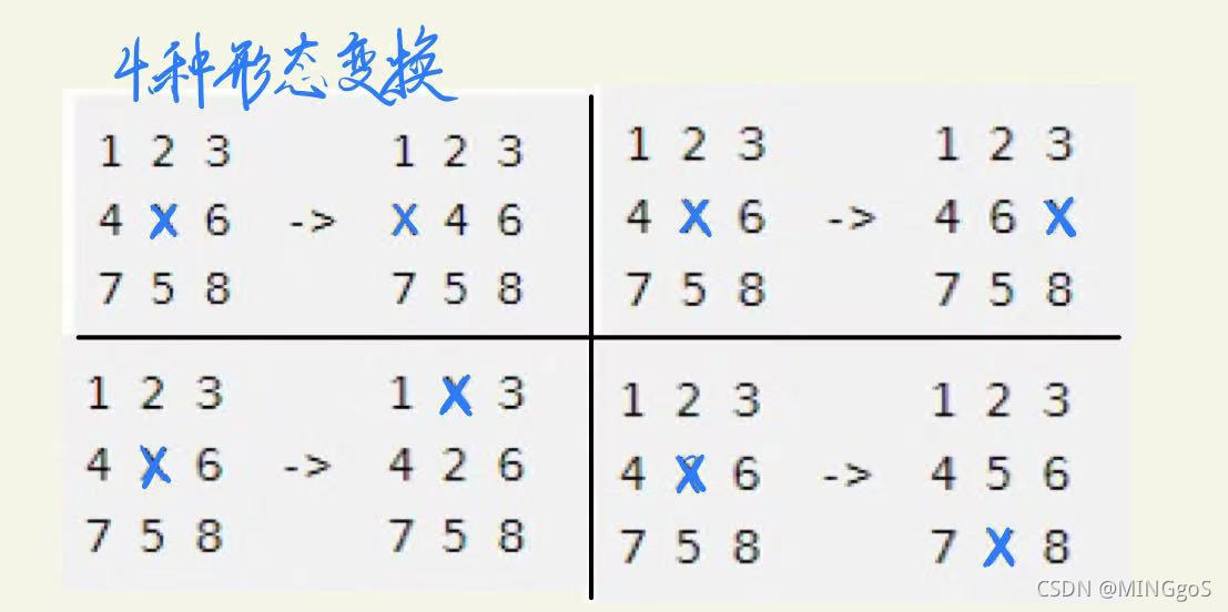
可以将矩阵转换为字符串,用字符串来表示矩阵当前的状态
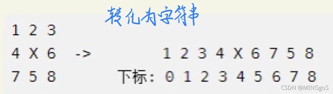
转换方法
1
2
| queue<string> q;
unordered_map<string, int> d;
|
1
2
3
4
5
6
7
8
9
10
11
12
13
14
15
16
17
18
19
20
21
22
23
24
25
26
27
28
29
30
31
32
33
34
35
36
37
38
39
40
41
42
43
44
45
46
47
48
49
50
51
52
53
54
55
56
57
58
59
60
61
62
63
64
65
66
67
68
69
70
71
72
73
74
75
76
| #include<iostream>
#include<algorithm>
#include<unordered_map>
#include<queue>
using namespace std;
int bfs(string start)
{
string end = "12345678x";
queue<string> q;
unordered_map<string, int> d;
q.push(start);
d[start] = 0;
int dx[4] = {-1, 0, 1, 0};
int dy[4] = {0, 1, 0, -1};
while(q.size())
{
auto t = q.front();
q.pop();
int distance = d[t];
if(t == end) return distance;
int k = t.find('x');
int x = k / 3, y = k % 3;
for(int i = 0; i < 4; i ++ )
{
int a = x + dx[i], b = y + dy[i];
if(a >= 0 && a < 3 && b >= 0 && b < 3)
{
swap(t[k], t[a * 3 + b]);
if(!d.count(t))
{
d[t] = distance + 1;
q.push(t);
}
swap(t[a * 3 + b], t[k]);
}
}
}
return -1;
}
int main()
{
string start;
for(int i = 0; i < 9; i ++ )
{
char c;
cin >> c;
start += c;
}
cout << bfs(start) << endl;
return 0;
}
|
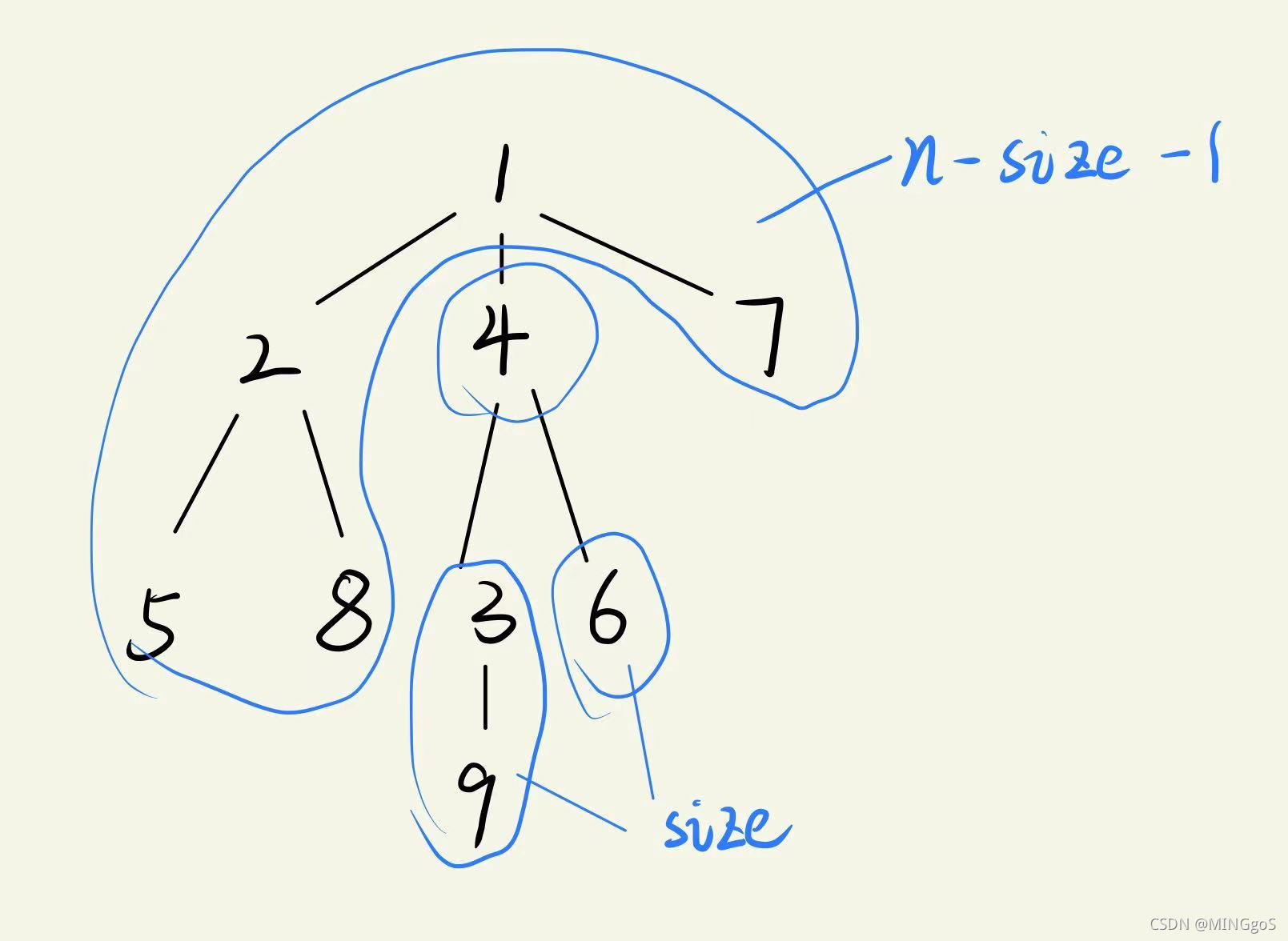
AcWing 846. 树的重心
dfs(4)时,节点4有3,6两个子节点,两个子节点所在的连通块的节点数加起来的值为size
节点4的父节点1所在连通块的节点数为n - size - 1
每个节点删去后的连通块节点数量最大值为size = max(size, n - size - 1),
找出使得连通块的节点数量最大值最小的点,这个点就是树的重心,利用一个全局变量ans来记录最小值,更新方式为ans = min(ans, size)
1
2
3
4
5
6
7
8
9
10
11
12
13
14
15
16
17
18
19
20
21
22
23
24
25
26
27
28
29
30
31
32
33
34
35
36
37
38
39
40
41
42
43
44
45
46
47
48
49
50
51
52
53
54
55
56
57
58
59
60
61
62
63
64
65
66
67
68
| #include<iostream>
#include<cstring>
#include<cstdio>
#include<algorithm>
using namespace std;
const int N = 1e5 + 10, M = 2 * N;
int n;
int h[N], e[M], ne[M], idx;
int ans = N;
bool st[N];
void add(int a, int b)
{
e[idx] = b, ne[idx] = h[a], h[a] = idx ++ ;
}
int dfs(int u)
{
st[u] = true;
int size = 0, sum = 0;
for(int i = h[u]; i != -1; i = ne[i])
{
int j = e[i];
if(st[j]) continue;
int s = dfs(j);
size = max(size, s);
sum += s;
}
size = max(size, n - sum - 1);
ans = min(ans, size);
return sum + 1;
}
int main()
{
scanf("%d", &n);
memset(h, -1, sizeof h);
for(int i = 0; i < n - 1; i ++ )
{
int a, b;
scanf("%d%d", &a, &b);
add(a, b), add(b, a);
}
dfs(1);
printf("%d\n", ans);
return 0;
}
|
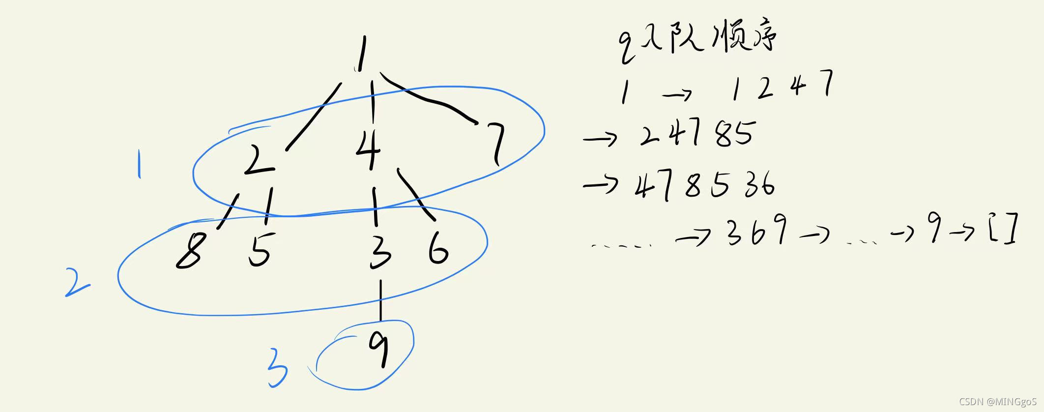
AcWing 847. 图中点的层次
1
2
3
4
5
6
7
8
9
10
11
12
13
14
15
16
17
18
19
20
21
22
23
24
25
26
27
28
29
30
31
32
33
34
35
36
37
38
39
40
41
42
43
44
45
46
47
48
49
50
51
52
53
54
55
56
57
58
59
| #include<iostream>
#include<cstring>
#include<algorithm>
#include<queue>
using namespace std;
const int N = 1e5 + 10;
queue<int> que;
int n, m;
int h[N], e[N], ne[N], idx;
int d[N], q[N];
void add(int a, int b)
{
e[idx] = b, ne[idx] = h[a], h[a] = idx ++ ;
}
int bfs()
{
que.push(1);
memset(d, -1, sizeof d);
d[1] = 0;
while(!que.empty())
{
int t = que.front();
que.pop();
for(int i = h[t]; i != -1; i = ne[i])
{
int j = e[i];
if(d[j] == -1)
{
d[j] = d[t] + 1;
que.push(j);
}
}
}
return d[n];
}
int main()
{
cin >> n >> m;
memset(h, -1, sizeof h);
for(int i = 0; i < m; i ++ )
{
int a, b;
cin >> a >> b;
add(a, b);
}
cout << bfs() << endl;
return 0;
}
|
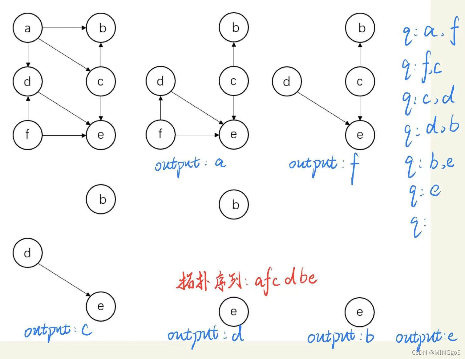
AcWing 848. 有向图的拓扑序列
将入度为0的节点入队,并将这个节点的子节点入度都减一,如果入度为0,就将节点入队,如此循环,直至所有节点都入队为止。
1
2
3
4
5
6
7
8
9
10
11
12
13
14
15
16
17
18
19
20
21
22
23
24
25
26
27
28
29
30
31
32
33
34
35
36
37
38
39
40
41
42
43
44
45
46
47
48
49
50
51
52
53
54
55
56
57
58
59
60
61
62
63
| #include<iostream>
#include<cstring>
using namespace std;
const int N = 1e5 + 10;
int n, m;
int h[N], ne[N], e[N], idx;
int q[N], d[N];
void add(int a, int b)
{
e[idx] = b, ne[idx] = h[a], h[a] = idx ++ ;
}
bool topSort()
{
int hh = 0, tt = -1;
for(int i = 1; i <= n; i ++ )
if(!d[i])
q[ ++ tt] = i;
while(hh <= tt)
{
int t = q[hh ++ ];
for(int i = h[t]; i != -1; i = ne[i])
{
int j = e[i];
d[j] --;
if(d[j] == 0) q[ ++ tt] = j;
}
}
return tt == n - 1;
}
int main()
{
cin >> n >> m;
memset(h, -1, sizeof h);
for(int i = 0; i < m; i ++ )
{
int a, b;
cin >> a >> b;
add(a, b);
d[b] ++ ;
}
if(topSort())
{
for(int i = 0; i < n; i ++ ) printf("%d ", q[i]);
puts("");
}
else cout << -1 << endl;
return 0;
}
|
AcWing 849. Dijkstra求最短路 I
Dijkstra算法介绍
Dijkstra的主要特点是以起始点为中心向外层层拓展(广度优先搜索思想),直到拓展到终点为止。
算法特点:
迪科斯彻算法使用了广度优先搜索解决赋权有向图或者无向图的单源最短路径问题,算法最终得到一个最短路径树。该算法常用于路由算法或者作为其他图算法的一个子模块。
算法的思路
Dijkstra算法采用的是一种贪心的策略,声明一个数组dis来保存源点到各个顶点的最短距离和一个保存已经找到了最短路径的顶点的集合:T,初始时,原点 s 的路径权重被赋为 0 (dis[s] = 0)。若对于顶点 s 存在能直接到达的边(s,m),则把dis[m]设为w(s, m),同时把所有其他(s不能直接到达的)顶点的路径长度设为无穷大。初始时,集合T只有顶点s。
然后,从dis数组选择最小值,则该值就是源点s到该值对应的顶点的最短路径,并且把该点加入到T中,OK,此时完成一个顶点,
然后,我们需要看看新加入的顶点是否可以到达其他顶点并且看看通过该顶点到达其他点的路径长度是否比源点直接到达短,如果是,那么就替换这些顶点在dis中的值。
然后,又从dis中找出最小值,重复上述动作,直到T中包含了图的所有顶点。
算法核心:松弛操作
1
2
3
4
5
6
7
8
9
10
11
12
13
14
15
16
17
|
for(int i = 0; i < n; i ++ )
{
int t = - 1;
for(int j = 1; j <= n; j ++ )
if(!st[j] && (t == -1 || dist[t] > dist[j]))
t = j;
st[t] = true;
for(int j = 1; j <= n; j ++ )
dist[j] = min(dist[j], dist[t] + g[t][j]);
}
|
过程图解
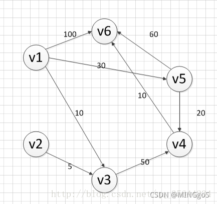
距离更新过程:
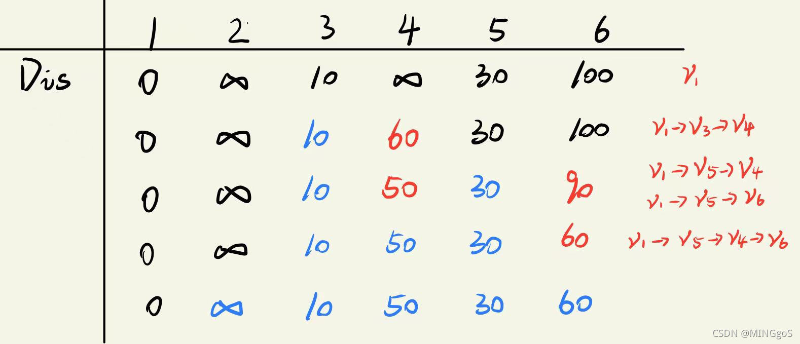
总结起来就是:每次选一个点,更新邻点,循环$n-1$次就可以了
时间复杂度$O(n \cdot n)$
1
2
3
4
5
6
7
8
9
10
11
12
13
14
15
16
17
18
19
20
21
22
23
24
25
26
27
28
29
30
31
32
33
34
35
36
37
38
39
40
41
42
43
44
45
46
47
48
49
50
51
52
53
54
55
56
57
58
59
60
| #include<iostream>
#include<cstring>
#include<algorithm>
using namespace std;
const int N = 510;
int n, m;
int g[N][N];
int dist[N];
bool st[N];
int dijkstra()
{
memset(dist, 0x3f, sizeof dist);
dist[1] = 0;
for(int i = 0; i < n; i ++ )
{
int t = - 1;
for(int j = 1; j <= n; j ++ )
if(!st[j] && (t == -1 || dist[t] > dist[j]))
t = j;
st[t] = true;
for(int j = 1; j <= n; j ++ )
dist[j] = min(dist[j], dist[t] + g[t][j]);
}
if(dist[n] == 0x3f3f3f3f) return -1;
return dist[n];
}
int main()
{
scanf("%d%d", &n, &m);
memset(g, 0x3f, sizeof g);
while(m --)
{
int a, b, c;
scanf("%d%d%d", &a, &b, &c);
g[a][b] = min(g[a][b], c);
}
int t = dijkstra();
printf("%d\n", t);
return 0;
}
|
AcWing 850. Dijkstra求最短路 II
堆优化的主要思想就是使用一个优先队列(就是每次弹出的元素一定是整个队列中最小的元素)来代替最近距离的查找,用邻接表代替邻接矩阵,这样可以大幅度节约时间开销。
在这里有几个细节需要处理:
-
首先来讲,优先队列的数据类型应该是怎样的呢?
我们知道优先队列应该用于快速寻找距离最近的点。由于优先队列只是将最小的那个元素排在前面,因此我们应该定义一种数据类型,使得它包含该节点的编号以及该节点当前与起点的距离。这里使用pair数组来储存。
-
我们应该在什么时候对队列进行操作呢?
队列操作的地方,首先就是搜索刚开始,要为起点赋初始值,此时必须将起点加入优先队列中。该队列元素的节点编号为起点的编号,该节点当前与起点的距离为0。
-
那么如果一个节点到起点的最短距离通过其他的运算流程发生了变化,那么如何处理队列中的那个已经存入的元素?
事实上,你不需要理会队列中的元素,而是再存入一个就行了。因为如果要发生变化,只能将节点与起点之间的距离变得更小,而优先队列恰好是先让最小的那个弹出。
因此,轮到某一个队列元素弹出的时候,如果有多个元素的节点编号相同,那么被弹出的一定是节点编号最小的一个。等到后面再遇到这个节点编号的时候,我们只需要将它忽略掉就行了
时间复杂度$O(m log n)$
1
2
3
4
5
6
7
8
9
10
11
12
13
14
15
16
17
18
19
20
21
22
23
24
25
26
27
28
29
30
31
32
33
34
35
36
37
38
39
40
41
42
43
44
45
46
47
48
49
50
51
52
53
54
55
56
57
58
59
60
61
62
63
64
65
66
67
68
69
70
71
72
73
74
| #include<iostream>
#include<cstring>
#include<algorithm>
#include<queue>
using namespace std;
typedef pair<int, int> PII;
const int N = 1e6 + 10;
int n, m;
int h[N], e[N], w[N], ne[N], idx;
int dist[N];
bool st[N];
void add(int a, int b, int c)
{
e[idx] = b, w[idx] = c, ne[idx] = h[a], h[a] = idx ++;
}
int dijkstra()
{
memset(dist, 0x3f, sizeof dist);
dist[1] = 0;
priority_queue<PII, vector<PII>, greater<PII>> heap;
heap.push({0, 1});
while(heap.size())
{
auto t = heap.top();
heap.pop();
int ver = t.second, distance = t.first;
if(st[ver]) continue;
st[ver] = true;
for(int i = h[ver]; i != -1; i = ne[i])
{
int j = e[i];
if(dist[j] > distance + w[i])
{
dist[j] = distance + w[i];
heap.push({dist[j], j});
}
}
}
if(dist[n] == 0x3f3f3f3f) return -1;
return dist[n];
}
int main()
{
scanf("%d%d", &n, &m);
memset(h, -1, sizeof h);
while(m -- )
{
int a, b, c;
scanf("%d%d%d", &a, &b, &c);
add(a, b, c);
}
int t = dijkstra();
printf("%d\n", t);
return 0;
}
|
AcWing 853. 有边数限制的最短路
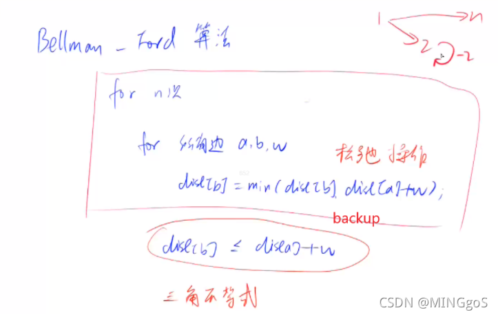
Bellman-Ford算法的优点是可以发现负圈,缺点是时间复杂度比Dijkstra算法高。
而SPFA算法是使用队列优化的Bellman-Ford版本,其在时间复杂度和编程难度上都比其他算法有优势。
参考文献
1
2
3
4
5
6
7
8
9
10
11
12
13
14
15
16
17
18
19
20
21
22
23
24
25
26
27
28
29
30
31
32
33
34
35
36
37
38
39
40
41
42
43
44
45
46
47
48
49
50
51
52
| #include<iostream>
#include<algorithm>
#include<cstring>
using namespace std;
const int N = 510, M = 1e4 + 10;
int n, m, k;
int dist[N], backup[N];
struct Edge
{
int a, b, w;
}edges[M];
int bellman_ford()
{
memset(dist, 0x3f, sizeof dist);
dist[1] = 0;
for(int i=0; i < k; i++)
{
memcpy(backup, dist, sizeof dist);
for(int j = 0; j < m; j ++)
{
int a = edges[j].a, b = edges[j].b, w = edges[j].w;
dist[b] = min(dist[b], backup[a] + w);
}
}
if(dist[n] > 0x3f3f3f3f / 2) return -1;
return dist[n];
}
int main()
{
scanf("%d%d%d", &n, &m, &k);
for(int i=0; i<m; i++)
{
int a, b, w;
scanf("%d%d%d", &a, &b, &w);
edges[i] = {a, b, w};
}
int t = bellman_ford();
if(t == -1) puts("impossible");
else printf("%d\n", t);
return 0;
}
|
AcWing 851. spfa求最短路
1
2
3
4
5
6
7
8
9
10
11
12
13
14
15
16
17
18
19
20
21
22
23
24
25
26
27
28
29
30
31
32
33
34
35
36
37
38
39
40
41
42
43
44
45
46
47
48
49
50
51
52
53
54
55
56
57
58
59
60
61
62
63
64
65
66
67
68
69
70
71
72
73
74
| #include<iostream>
#include<cstring>
#include<algorithm>
#include<queue>
using namespace std;
const int N = 1e5 + 10;
int n, m;
int h[N], w[N], e[N], ne[N], idx;
int dist[N];
bool st[N];
void add(int a, int b, int c)
{
e[idx] = b, w[idx] = c, ne[idx] = h[a], h[a] = idx ++ ;
}
int spfa()
{
memset(dist, 0x3f, sizeof dist);
dist[1] = 0;
queue<int> q;
q.push(1);
st[1] = true;
while(q.size())
{
int t = q.front();
q.pop();
st[t] = false;
for(int i = h[t]; i != -1; i = ne[i])
{
int j = e[i];
if(dist[j] > dist[t] + w[i])
{
dist[j] = dist[t] + w[i];
if(!st[j])
{
q.push(j);
st[j] = true;
}
}
}
}
if(dist[n] == 0x3f3f3f3f) return -1;
return dist[n];
}
int main()
{
scanf("%d%d", &n, &m);
memset(h, -1, sizeof h);
while(m -- )
{
int a, b, c;
scanf("%d%d%d", &a, &b, &c);
add(a, b, c);
}
int t = spfa();
if(t == -1) puts("impossible");
else printf("%d\n", t);
return 0;
}
|
AcWing 852. spfa判断负环
1
2
3
4
5
6
7
8
9
10
11
12
13
14
15
16
17
18
19
20
21
22
23
24
25
26
27
28
29
30
31
32
33
34
35
36
37
38
39
40
41
42
43
44
45
46
47
48
49
50
51
52
53
54
55
56
57
58
59
60
61
62
63
64
65
66
67
68
69
70
71
72
73
74
| #include<iostream>
#include<cstring>
#include<algorithm>
#include<queue>
using namespace std;
const int N = 1e5 + 10;
int n, m;
int h[N], w[N], e[N], ne[N], idx;
int dist[N], cnt[N];
bool st[N];
void add(int a, int b, int c)
{
e[idx] = b, w[idx] = c, ne[idx] = h[a], h[a] = idx ++;
}
int spfa()
{
queue<int> q;
for(int i = 1; i <= n; i ++ )
{
st[i] = true;
q.push(i);
}
while(q.size())
{
int t = q.front();
q.pop();
st[t] = false;
for(int i = h[t]; i != -1; i = ne[i])
{
int j = e[i];
if(dist[j] > dist[t] + w[i])
{
dist[j] = dist[t] + w[i];
cnt[j] = cnt[t] + 1;
if(cnt[j] >= n) return true;
if(!st[j])
{
q.push(j);
st[j] = true;
}
}
}
}
return false;
}
int main()
{
scanf("%d%d", &n, &m);
memset(h, -1, sizeof h);
while(m--)
{
int a, b, c;
scanf("%d%d%d", &a, &b, &c);
add(a, b, c);
}
if(spfa()) puts("Yes");
else puts("No");
return 0;
}
|
AcWing 854. Floyd求最短路
基本思想:
弗洛伊德算法定义了两个二维矩阵:
矩阵D记录顶点间的最小路径
例如D[0][3]= 10,说明顶点0 到 3 的最短路径为10;
矩阵P记录顶点间最小路径中的中转点
例如P[0][3]= 1 说明,0 到 3的最短路径轨迹为:0 -> 1 -> 3。
它通过3重循环,k为中转点,v为起点,w为终点,循环比较D[v][w] 和D[v][k] + D[k][w]最小值,如果D[v][k] + D[k][w] 为更小值,则把D[v][k] + D[k][w] 覆盖保存在D[v][w]中。
算法核心
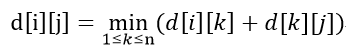
过程图解
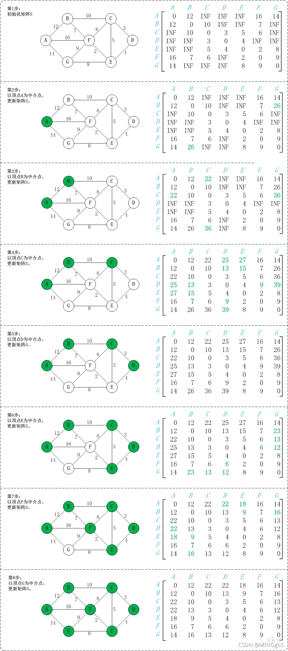
时间复杂度$O(n \cdot n \cdot n)$
1
2
3
4
5
6
7
8
9
10
11
12
13
14
15
16
17
18
19
20
21
22
23
24
25
26
27
28
29
30
31
32
33
34
35
36
37
38
39
40
41
42
43
44
| #include<iostream>
#include<algorithm>
using namespace std;
const int N = 210, INF = 1e9;
int n, m, Q;
int d[N][N];
void floyd()
{
for(int k = 1; k <= n; k ++ )
for(int i = 1; i <= n; i ++ )
for(int j = 1; j <= n; j ++ )
d[i][j] = min(d[i][j], d[i][k] + d[k][j]);
}
int main()
{
cin >> n >> m >> Q;
for(int i = 1; i <= n; i ++ )
for(int j = 1; j <= n; j ++ )
if(i == j) d[i][j] = 0;
else d[i][j] = INF;
while(m -- )
{
int a, b, w;
cin >> a >> b >> w;
d[a][b] = min(d[a][b], w);
}
floyd();
while(Q -- )
{
int a, b;
cin >> a >> b;
if(d[a][b] > INF / 2) puts("impossible");
else cout << d[a][b];
}
return 0;
}
|
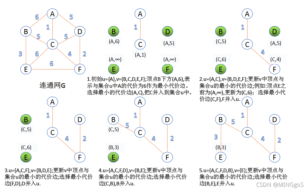
AcWing 858. Prim算法求最小生成树
- 连通图:在无向图中,若任意两个顶点vivi与vjvj都有路径相通,则称该无向图为连通图。
- 强连通图:在有向图中,若任意两个顶点vivi与vjvj都有路径相通,则称该有向图为强连通图。
- 连通网:在连通图中,若图的边具有一定的意义,每一条边都对应着一个数,称为权;权代表着连接连个顶点的代价,称这种连通图叫做连通网。
- 生成树:一个连通图的生成树是指一个连通子图,它含有图中全部n个顶点,但只有足以构成一棵树的n-1条边。一颗有n个顶点的生成树有且仅有n-1条边,如果生成树中再添加一条边,则必定成环。
- 最小生成树:在连通网的所有生成树中,所有边的代价和最小的生成树,称为最小生成树。
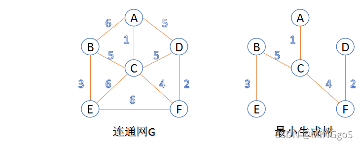
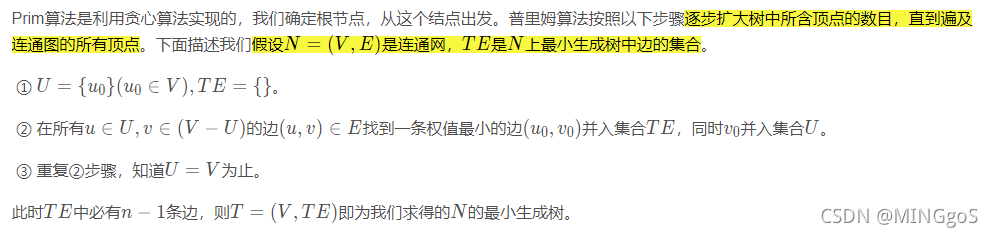
Prim过程图解:
1
2
3
4
5
6
7
8
9
10
11
12
13
14
15
16
17
18
19
20
21
22
23
24
25
26
27
28
29
30
31
32
33
34
35
36
37
38
39
40
41
42
43
44
45
46
47
48
49
50
51
52
53
54
55
56
57
58
59
60
61
| #include<iostream>
#include<cstring>
#include<algorithm>
using namespace std;
const int N = 510, INF = 0x3f3f3f3f;
int n, m;
int g[N][N];
int dist[N];
bool st[N];
int prim()
{
memset(dist, 0x3f, sizeof dist);
int res = 0;
for(int i = 0; i < n; i ++ )
{
int t = -1;
for(int j = 1; j <= n; j ++ )
if(!st[j] && (t == -1 || dist[t] > dist[j]))
t = j;
if(i && dist[t] == INF) return INF;
if(i) res += dist[t];
for(int j = 1; j <= n; j ++ )
dist[j] = min(dist[j], g[t][j]);
st[t] = true;
}
return res;
}
int main()
{
scanf("%d%d", &n, &m);
memset(g, 0x3f, sizeof g);
while(m--)
{
int a, b, c;
scanf("%d%d%d", &a, &b, &c);
g[a][b] = g[b][a] = min(g[a][b], c);
}
int t = prim();
if(t == INF) puts("impossible");
else printf("%d\n", t);
return 0;
}
|
AcWing 859. Kruskal算法求最小生成树
此算法可以称为“加边法”,初始最小生成树边数为0
利用并查集来维护每条边所属的集合
每迭代一次就选择一条满足条件的最小代价边,加入到最小生成树的边集合里。
- 把图中的所有边按边权从小到大排序;
- 把图中的n个顶点看成独立的n棵树组成的森林;
- 按权值从小到大选择边,所选的边连接的两个顶点应属于两个不同的集合,并将这两颗集合合并。如果所选的两个点属于同一个集合,那么将这条边加入集合后,将会形成一个环,不符合树的定义。
- 重复(3),直到所有顶点都在一颗树内或者有n-1条边为止。
Kruskal过程图解:
1
2
3
4
5
6
7
8
9
10
11
12
13
14
15
16
17
18
19
20
21
22
23
24
25
26
27
28
29
30
31
32
33
34
35
36
37
38
39
40
41
42
43
44
45
46
47
48
49
50
51
52
53
54
55
56
57
58
59
| #include<iostream>
#include<algorithm>
using namespace std;
const int N = 2e5 + 10;
int n, m;
int p[N];
struct Edge
{
int a, b, w;
bool operator< (const Edge &W)const
{
return w < W.w;
}
}edges[N];
int find(int x)
{
if(p[x] != x) p[x] = find(p[x]);
return p[x];
}
int main()
{
scanf("%d%d", &n, &m);
for(int i = 0; i < m; i ++ )
{
int a, b, w;
scanf("%d%d%d", &a, &b, &w);
edges[i] = {a, b, w};
}
sort(edges, edges + m);
for(int i = 1; i <= n; i ++ ) p[i] = i;
int res = 0, cnt = 0;
for(int i = 0; i < m; i ++ )
{
int a = edges[i].a, b = edges[i].b, w = edges[i].w;
a = find(a), b = find(b);
if(a != b)
{
p[a] = b;
res += w;
cnt ++;
}
}
if(cnt < n - 1) puts("impossible");
else printf("%d\n", res);
return 0;
}
|
AcWing 860. 染色法判定二分图
奇数环:由奇数条边形成的一个环
把一个图的顶点划分为两个不相交子集 ,使得每一条边都分别连接两个集合中的顶点。如果存在这样的划分,则此图为一个二分图
二分图可能含有偶数环,但一定没有奇数环,一下图形都是二分图
利用dfs对图中的点进行染色,可以判断该图是否为二分图
1
2
3
4
5
6
7
8
9
10
11
12
13
14
15
16
17
18
19
20
21
22
23
24
25
26
27
28
29
30
31
32
33
34
35
36
37
38
39
40
41
42
43
44
45
46
47
48
49
50
51
52
53
54
55
56
57
58
59
60
61
62
63
64
65
66
67
68
69
70
71
| #include<iostream>
#include<cstring>
using namespace std;
const int N = 1e5 + 10, M = 2e5 + 10;
int n, m;
int h[N], e[M], ne[M], idx;
int color[N];
void add(int a, int b)
{
e[idx] = b, ne[idx] = h[a], h[a] = idx ++ ;
}
bool dfs(int u, int c)
{
color[u] = c;
for(int i = h[u]; i != -1; i = ne[i])
{
int j = e[i];
if(!color[j])
{
if(!dfs(j, 3 - c)) return false;
}
else if(color[j] == c) return false;
}
return true;
}
int main()
{
scanf("%d%d", &n, &m);
memset(h, -1, sizeof h);
while(m -- )
{
int a, b;
scanf("%d%d", &a, &b);
add(a, b), add(b, a);
}
bool flag = true;
for(int i = 1; i <= n; i ++ )
if(!color[i])
{
if(!dfs(i, 1))
{
flag = false;
break;
}
}
if(flag) puts("Yes");
else puts("No");
return 0;
}
|
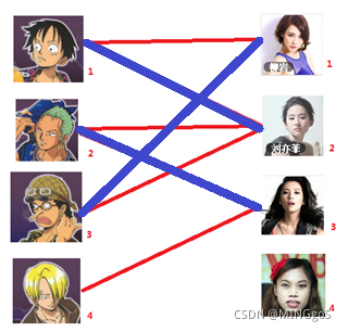
AcWing 861. 二分图的最大匹配
匈牙利算法几乎是二分图匹配的核心算法,除了二分图多重匹配外均可使用
先试着给1号男生找妹子,发现第一个和他相连的1号女生还名花无主,连上一条蓝线
接着给2号男生找妹子,发现第一个和他相连的2号女生名花无主
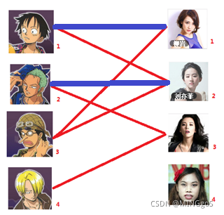
接下来是3号男生,很遗憾1号女生已经有主了,怎么办呢?
我们试着给之前1号女生匹配的男生(也就是1号男生)另外分配一个妹子。
(黄色表示这条边被临时拆掉)
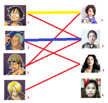
与1号男生相连的第二个女生是2号女生,但是2号女生也有主了
我们再试着给2号女生的原配重新找个妹子
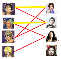
2号男生可以找3号妹子~~~~~~~~ 1号男生可以找2号妹子了~~~~~~~~ 3号男生可以找1号妹子
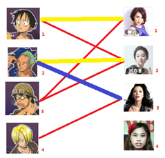
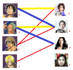
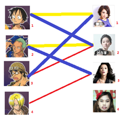
结果就是这样
1
2
3
4
5
6
7
8
9
10
11
12
13
14
15
16
17
18
19
20
21
22
23
24
25
26
27
28
29
30
31
32
33
34
35
36
37
38
39
40
41
42
43
44
45
46
47
48
49
50
51
52
53
54
55
56
57
58
59
60
61
62
63
64
65
66
67
68
69
| #include<iostream>
#include<cstring>
using namespace std;
const int N = 510, M = 1e5 + 10;
int n1, n2, m;
int h[N], e[M], ne[M], idx;
int match[N];
bool st[N];
void add(int a, int b)
{
e[idx] = b, ne[idx] = h[a], h[a] = idx ++;
}
bool find(int x)
{
for(int i = h[x]; i != -1; i = ne[i])
{
int j = e[i];
if(!st[j])
{
st[j] = true;
if(match[j] == 0 || find(match[j]))
{
match[j] = x;
return true;
}
}
}
return false;
}
int main()
{
scanf("%d%d%d", &n1, &n2, &m);
memset(h, -1, sizeof h);
while(m --)
{
int a, b;
scanf("%d%d", &a, &b);
add(a, b);
}
int res = 0;
for(int i = 1; i <= n1; i ++ )
{
memset(st, false, sizeof st);
if(find(i)) res ++;
}
printf("%d\n", res);
return 0;
}
|